Method for persistent topological features extraction of schizophrenia patients’ electroencephalography signal based on persistent homology
 Guangxing Guo1,2,3†,
  Yanli Zhao4†, Chenxu Liu5,
  Yongcan Fu5, Xinhua Xi5, Lizhong Jin6, Dongli Shi5, Lin Wang5, Yonghong Duan3, Jie Huang4,
  Shuping Tan4* and
  Guimei Yin5*
- 1College of Geography Science, Taiyuan Normal University, Jinzhong, China
- 2Institute of Big Data Analysis Technology and Application, Taiyuan Normal University, Jinzhong, China
- 3College of Resource and Environment, Shanxi Agricultural University, Taigu, China
- 4Psychiatry Research Center, Beijing Huilongguan Hospital, Peking University Huilongguan Clinical Medical School, Beijing, China
- 5Laboratory of Data Mining and Machine Learning, College of Computer Science and Technology, Taiyuan Normal University, Jinzhong, China
- 6College of Applied Science, Taiyuan University of Science and Technology, Taiyuan, China
With the development of network science and graph theory, brain network research has unique advantages in explaining those mental diseases, the neural mechanism of which is unclear. Additionally, it can provide a new perspective in revealing the pathophysiological mechanism of brain diseases from the system level. The selection of threshold plays an important role in brain networks construction. There are no generally accepted criteria for determining the proper threshold. Therefore, based on the topological data analysis of persistent homology theory, this study developed a multi-scale brain network modeling analysis method, which enables us to quantify various persistent topological features at different scales in a coherent manner. In this method, the Vietoris–Rips filtering algorithm is used to extract dynamic persistent topological features by gradually increasing the threshold in the range of full-scale distances. Subsequently, the persistent topological features are visualized using barcodes and persistence diagrams. Finally, the stability of persistent topological features is analyzed by calculating the Bottleneck distances and Wasserstein distances between the persistence diagrams. Experimental results show that compared with the existing methods, this method can extract the topological features of brain networks more accurately and improves the accuracy of diagnostic and classification. This work not only lays a foundation for exploring the higher-order topology of brain functional networks in schizophrenia patients, but also enhances the modeling ability of complex brain systems to better understand, analyze, and predict their dynamic behaviors.
Introduction
Topological data analysis (TDA) (Edelsbrunner and Harer, 2010; Ibekwe et al., 2014; Taylor et al., 2015) is related to data analysis, algebraic topology, computational geometry, computer science, and statistics. The main goal of TDA is to use geometry and topology theories to study the qualitative features of data. To achieve this, a precise definition of qualitative features and computational tools in specific practical applications is required. Theories ensure the stability and robustness of these features. One way to achieve this goal is using persistent homology (PH) in TDA (Aktas et al., 2019). Currently, researches on the application of PH to brain network analysis are gaining increasing attention (Lee et al., 2012; Caputi et al., 2021; Xu et al., 2021).
When processing and analyzing brain imaging data, a matrix representing the connection strength between nodes is generated, and a threshold is selected to binarize the matrix. Finally, the adjacency matrix is generated to construct brain networks. The selection of the threshold plays an important role in network construction because it affects the connection density and network topology (Khalid et al., 2014; Chung et al., 2015; Sizemore et al., 2018). Generally, there are three methods for network binarization (Telesford et al., 2011). First, when a connection density is selected as a single threshold, for example, the structure of networks is fully connected when is selected (Castro et al., 2011; Li and Fan, 2013), where N is the number of nodes in the networks. This implies that there are no isolated points in the networks. However, this method cannot be applied to real networks because it is suitable only for random networks. The second method involves using a predefined threshold space, wherein the threshold is selected indirectly, and statistical methods are usually use to eliminate the weak connections or pseudo connections. However, the process of threshold selection is complex and not universal when data is changed (Yin et al., 2020; Zhu et al., 2020). Moreover, some important information transmission may be deleted when the weak connections are deleted. The third method involves using a threshold space at condition limits; essentially, the brain network with small-world attributes is built on the selected threshold space. The construction of a random network requires a mean degree of nodes greater than 2lgN and the same number of nodes and degree of nodes as the original network.
Numerous new thresholding methods have been reported, such as the network’s minimum spanning tree, which builds an unbiased network. Minimum spanning tree is not sensitive to thresholds and density values, so it is considered a good method for network binarization. However, this unbiased network is extremely sparse, which results in several important local connections being ignored (Tewarie et al., 2015). A windowless method based on a thermonuclear Gaussian core has been reported (Huang et al., 2019; Jin et al., 2019). In this method, the false rapid changing states of brain connections in the networks are reduced, and the problem of high-frequency noise is solved when the sliding window method is applied to dynamic brain network analysis.
Although numerous methods have been proposed for selecting a threshold when the brain networks are constructed in different ways, the selection of a network threshold remains difficult because there is no consensus on the best strategy (van Wijk et al., 2010). Therefore, the PH theory in the TDA method was introduced into brain network analysis (Shnier et al., 2019; Caputi et al., 2021). The advantages of this method are that the construction of brain networks does not require binarization, the networks can be analyzed on full-scale, and persistent topological features in the brain networks can be extracted across multiple scales.
Background
We reviewed some fundamental notions and results from PH that are relevant to our work. For more mathematical introductions, see Zomorodian and Carlsson (2005), Adler et al. (2010), Otter et al. (2017), and Aktas et al. (2019).
Definition 1
Let a topological space U on set X be a subset on 2X, namely, U⊂2X, if the following conditions are met: (1) Φ,X⊂U; (2) u1,u2⊂U, u1∪u2⊂U; (3) u1,u2⊂U,u1∩u2⊂U; then, (X,U) is called the topological space of the finite set X (Horak et al., 2009; Edelsbrunner and Harer, 2010).
Definition 2
In the n-dimensional vector space Rn of the real number field, there are a set of vectors a0,a1,a2,⋯,an, which make {a1−a0,a2−a0,⋯,an−a0} linearly independent. We set up E = θ0a0 + θ1a1 + ⋯ + θnan|θ0 + θ1 + ⋯ + θn = 1,θi > 0, and the point set E is called an n-dimensional simplex (Horak et al., 2009).
A zero-dimensional simplex is a point, a one-dimensional simplex is a line segment, a two-dimensional simplex is a triangle, and a three-dimensional simplex is a three-dimensional triangle.
Definition 3
Let K be a finite set of simplexes, if the following conditions are met: (1) If σ ∈ K, then any face of any simplex in K still belongs to K. (2) For σ1,σ2 ∈ K, if σ1∩σ2 is an empty set or σ1∩σ2 is on the common side of σ1 and σ2, then K is called a simple complex (Horak et al., 2009). The maximum dimension of a simplex in simplex K is called the dimension of K, expressed as
Definition 4
For a point cloud aggregation X, let d(,) represent the distance between two points in a point cloud set. ℛ(X,ε) is a Vietoris–Rips (VIPs) complex (Carlsson, 2009) if and only if its k-dimensional simplex [x0,x1,⋯,xk] satisfies d(xi,xj)≤ε, 0≤i,j≤k.
Full-scale brain network analysis model based on PH
The full-scale brain network analysis model designed in this study according to the PH data analysis method and the features of electroencephalography (EEG) signal processing is shown in Figure 1. First, the input of the model is the EEG time series signal, these electrical signals will convert to point clouds, see Section “From data to point clouds” for details. Second, according to Pearson correlation measure, the adjacency matrix of the nodes coordinate was constructed in this measure space, the construction process is shown in Section “Construction of the adjacency matrix.” Subsequently, the VIPs filtering algorithm is selected to calculate the persistent topology features of the network in Section “Filtering the brain network complexes,” and visualize it as barcodes and persistence diagrams in Section “Visualization of persistent topological features.” Finally, in Section “Stability analysis of persistent topological features,” according to the persistence graph stability theorem, the Bottleneck distance and Wasserstein distance are selected to analyze the stability of persistence features from the aspects of local details and global differences, and then determine the persistence topological features of networks. Section “Experiment and analysis” is the experimental part of the above process.
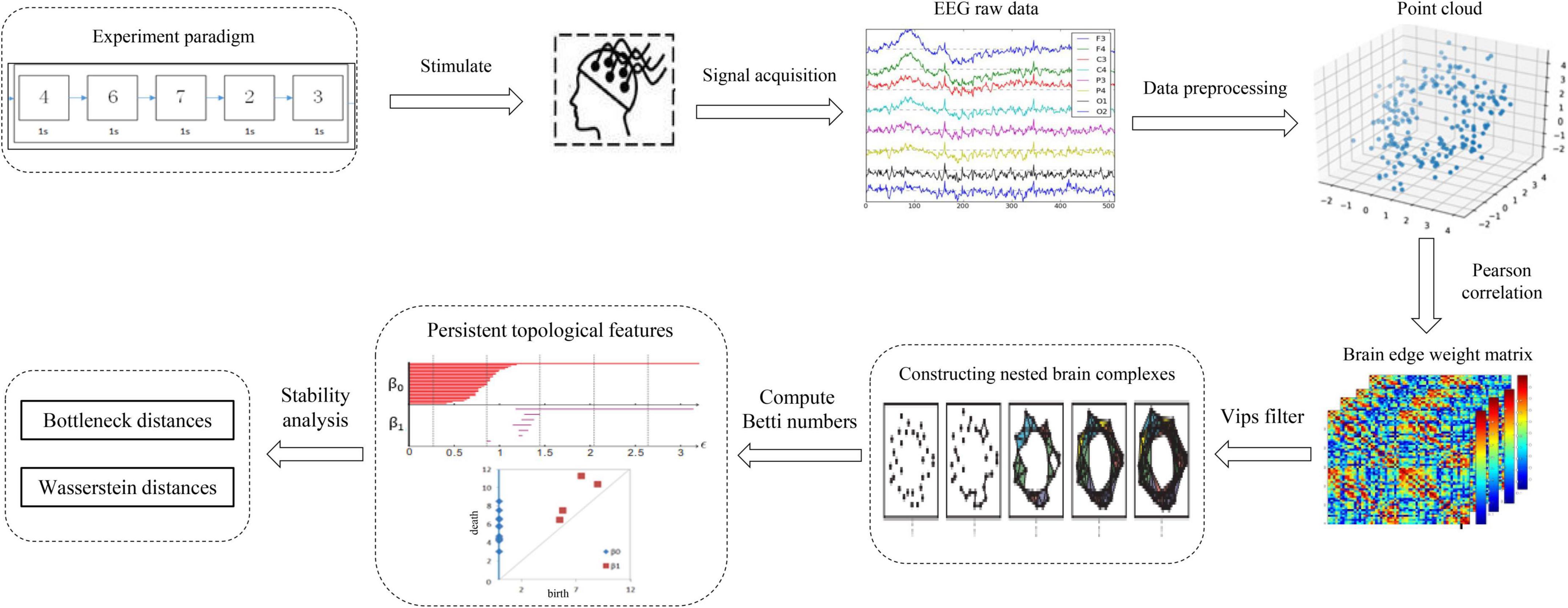
Figure 1. Framework of the full-scale brain network analysis model based on PH.
From data to point clouds
The preprocessed EEG time series signal is used as the input of the model, and the time series are transformed into points by down-sampling, and then into point clouds after defining the metric space and distance. However, selecting an appropriate distance for translate data points to point clouds is a key issue (Otter et al., 2017). The metric space in EEG data can choose distance metric, correlation metric, or synchronization metric. Scalp electrodes are often used as brain network nodes; however, the collected EEG signals are non-stationary owing to the volume conduction effect, and each node in the network has non-linear dynamic characteristics. Therefore, distance measurement is unsuitable. According to the preliminary experimental work of Zalesky et al. (2012), Pearson correlation is selected to measure the distance between nodes to construct an undirected weighted network. The detailed construction process will be introduced in Section “Construction of the simple complex in schizophrenia task-based data.”
Construction of the adjacency matrix
The preprocessed EEG time series signal was input into the model and the Pearson correlation measurement space was selected to construct the adjacent matrix for each channel data (i.e., point cloud) of the EEG signal. Based on the characteristics of the EEG signals, an undirected weighted network was constructed, and the electrode channels were taken as network nodes, thus signifying a one-dimensional simplex.
Filtering the brain network complexes
The process of constructing a nested brain network complex is the process of using PH filtering algorithm to filter. PH is divided into two parts: homology and persistence. Homology in group theory is a tool for classifying topological sets and measuring the specific structure of a simple complex. Persistence is used to extract all given ε persistent structures, that is, to obtain persistent topological features. Among the features, valuable features can be maintained for long durations, whereas noise can be maintained for short durations. This process is called PH. The key steps in constructing the complex are selecting the appropriate filtering threshold ε and filtering algorithm.
Selection of the filtering threshold
The selection of the filtering threshold ε is very important (Otter et al., 2017). The common method for this involves selecting different ε values to construct the complex and subsequently finding the ε value corresponding to the effective result. If ε is too small, then the complex may be the original point clouds or several edges of the point clouds. If ε is too large, the original point clouds could form a huge super-dimensional complex.
Selection of filtering algorithm
For different practical applications, different types of simple complexes with different attributes must be constructed. Some are easy to describe mathematically and easy to calculate, whereas others are simple but inefficient. For example, some common algorithms for constructing a simple complex are Cech complex algorithm (Espinoza et al., 2020), VIPs algorithm (Choudhary, 2017), alpha algorithm (Jamil and Kim, 2019), and witness algorithm (Guibas and Oudot, 2008). Based on graph filtering, the VIPs complex algorithm is suitable for complex brain networks in complex construction based on graph theory; furthermore, this algorithm has good performance in processing high-dimensional data. Therefore, the VIPs complex algorithm (Zomorodian and Graphics, 2010) was selected for filtering in this experiment.
Visualization of persistent topological features
When the VIPs filtering algorithm is used to calculate the persistent topological features of the network, with the change in filtering threshold ε, the topological features of the VIPs complex change. During the filtering process, changes in the network topology are visualized using barcodes or persistence diagrams (Carlsson et al., 2005; Ghrist, 2008). The filtering process is used primarily to calculate the p-dimensional Betti number interval [εbirthεdeath], where the εbirth is the start time of the p-dimensional hole in the simple complex and the εdeath is the time of its disappearance. Furthermore, they are also the start and end points of the barcode in the barcode’s visualization. These intervals are represented graphically as persistent barcodes, and the persistence diagrams are equivalent to barcodes. In the barcodes, the abscissa represents the time when the persistent features appear, that is, εbirth; whereas the ordinate represents the time εdeath when the persistent features disappear. The interval set [εbirthεdeath] obtained in the filtering process is considered as coordinates of the midpoint of the persistence diagrams, and all pairs of interval sets represent the coordinates to draw the persistence diagrams. The abscissa represents the filtering threshold ε, and the length of [εbirthεdeath] represents the length of the barcodes. The barcode with a large length represents the persistent topological feature, and the barcode with a short length or only one point represents noise. Correspondingly, the points far from the diagonal represent persistent features, whereas the points close to the diagonal represent noise in the persistence diagrams.
Stability analysis of persistent topological features
Stability analysis of topological features, i.e., the statistical analysis of barcodes, is a rapidly developing research direction (Lee et al., 2017). This requires the development of corresponding statistical methods and using persistence diagrams to compare and analyze. In the network matching problem, a persistence diagram is created for each network; subsequently, the persistence diagram is compared to obtain the similarity of the network (Agarwal and Sharathkumar, 2014). Currently, three methods can be used to solve the statistical analysis of barcodes (Otter et al., 2017). The first method involves studying the topological features of a random simple complex (Adler et al., 2010; Young et al., 2017). Essentially, when studying the PH, the random simple complex is considered an empty model and the experimental data is compared with it (Stolz, 2014). The second method, which is presently the most common method, involves studying the features of persistence diagrams in specific metric space. The third method involves mapping the space of the persistence diagram to a space suitable for statistical analysis and machine learning methods, such as Banach space (Bubenik, 2015; Bubenik and Dłotko, 2017; Kerber et al., 2017). Such methods include the use of algebraic functions, persistence diagrams and kernel techniques, and persistent landscapes in geometric function space. The second method, which is experiential and suitable for brain network analysis, was selected in this experiment.
The common stability metrics are the Bottleneck distance and Wasserstein distance. A small disturbance to the dataset that causes only a small change in the persistence diagrams before this standard indicates that this is a stable measurement standard.
Definition 5
Let p ∈ [1,∞), and the p-order Wasserstein distance (Zavlanos et al., 2008; Kerber et al., 2017) between two diagrams X and Y is defined as
where ∅:X→Y are mappings from X to Y. When p = ∞, distance d is a measure of a two-dimensional space, and the above formula is expressed as
where W∞[d∞] is the Bottleneck distance (Efrat et al., 2001).
The Bottleneck distance measures the maximum distance between the corresponding matching points of the two diagrams, which can capture large changes of persistence diagrams. The Wasserstein distance measures the total distance between the corresponding matching points of two diagrams, which can provide the overall change in similarity between persistence diagrams. In addition, it is sensitive to small changes in the persistence diagrams.
Experiment and analysis
Experimental data and preprocessing
The dataset used in this study was task-based EEG data; it was collected from Beijing Huilongguan Hospital. The experimental paradigm used the modified Sternberg’s short-term memory scanning task (SMST) (Manoach et al., 1999) paradigm (see Figure 2). The experimental processing was divided into three stages, namely, encoding, maintenance, and retrieval.
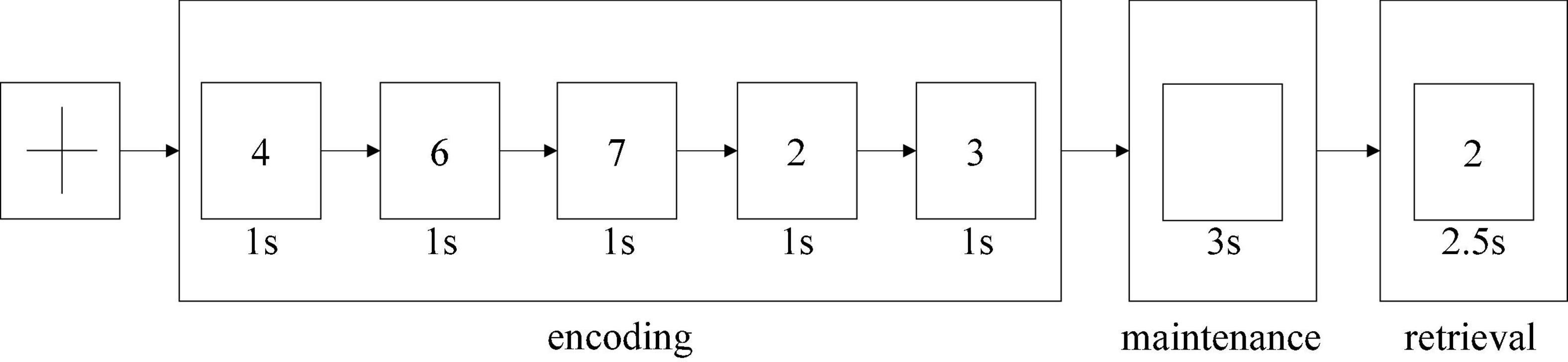
Figure 2. SMST paradigm.
The Sternberg’s short-term memory scanning task (SMST) paradigm (Sternberg, 1966; Jungeblut et al., 2021) is described in previous studies. Subjects were presented sets of 5 digits from 0 to 9 and were asked to memorize them. In each trial, an initial fixation was presented for 2 s; next, the 5 digits sets were presented for 1 s each (encoding phase) (Figure 2). Following a 3-s delay (maintenance phase), a probe stimulus was presented for 2.5 s (retrieval phase). Participants were asked to indicate whether the probe number was in the previous set of digits by pressing buttons. Probe digits that were present or absent from the encoding phase were presented 50 times each. The reaction time and probe identification accuracy were recorded. Trials in which the reaction time was less than 200 ms were excluded from the analysis.
The subjects came from the Schizophrenia Spectrum Disorder Project of Beijing Huilongguan Hospital. All patients were inpatients of Beijing Huilongguan Hospital and normal controls were recruited from the surrounding community and university. To select proper sample size, we have performed power analysis with G. PowerWin_3.1.9.3 software, and the parameter settings are as follows: effect size | ρ| was 0.5, significance level α was 0.05, power value 1 − β was 0.9. This yielded 34 individuals in per group. So we selected 35 individuals in this experiment. Thirty-five adult inpatients with a Diagnostic and Statistical Manual of Mental Disorders-IV (DSM-IV) (Segal, 2010) diagnosis of schizophrenia were recruited in the present study. Patients with a history of substance abuse within 6 months prior to the date of the experiment or additional neuropsychiatry diagnoses were excluded. Current clinical symptoms were assessed using positive and negative syndrome scale (PANSS) (Kay et al., 1987). An additional 35 normal control participants were recruited from the surrounding community through poster advertisements. Control subjects with a history of mental illness or substance abuse were excluded. There were no significant differences between the two groups with respect to age and sex through using with the double independent sample t-test method to compare (Table 1).
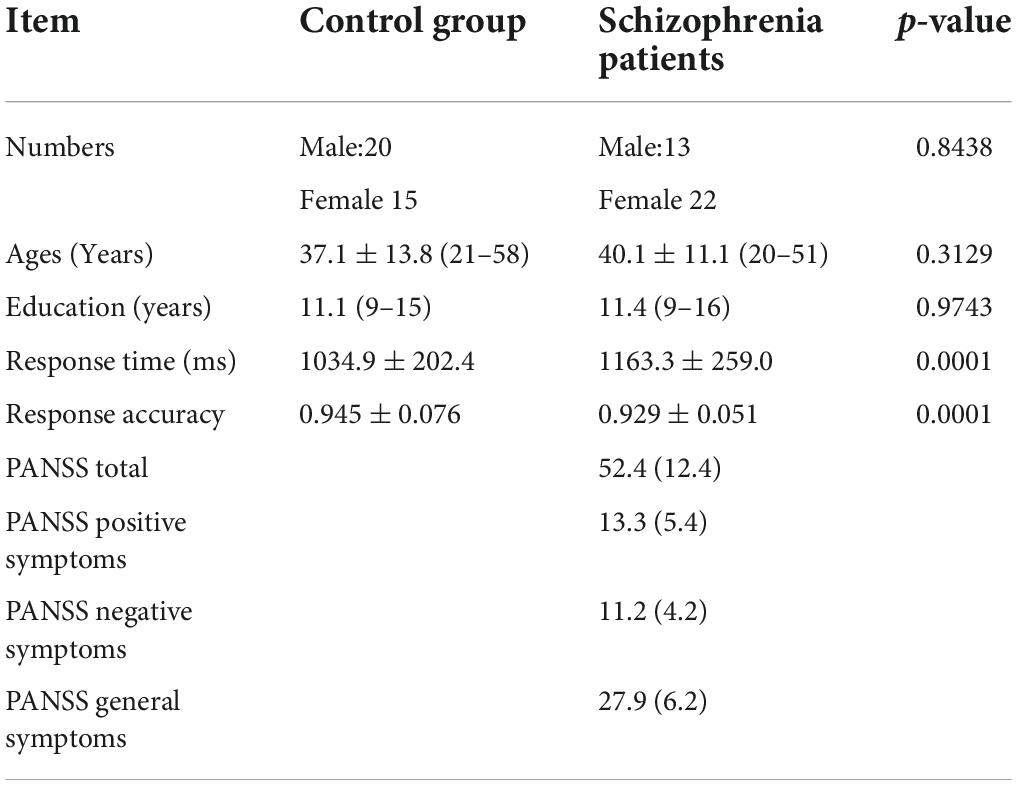
Table 1. Demographic and clinical characteristic of patients with schizophrenia and controls.
After re-reference, segmentation, removal of eye electric artifacts, and electromyography, the scale of network nodes was 60 and was divided into five bands, namely, θ (4–7 Hz), α (7–14 Hz), β1 (14–20 Hz), β2 (20–30 Hz), and γ (30–40 Hz) (Li et al., 2020).
Construction of the adjacency matrix based on PH
In the experiment, the construction of the adjacency matrix was based on the Pearson correlation (Benesty et al., 2009; Li et al., 2017) metric space, wherein the reciprocal of the Pearson correlation coefficient was taken as the weight of the connection between nodes and an undirected weighted network with dimensions of 60 × 60 was generated. The dynamic adjacency matrix constructed at different sparsity in the coding stage of working memory (WM) in schizophrenia is shown in Figure 3.
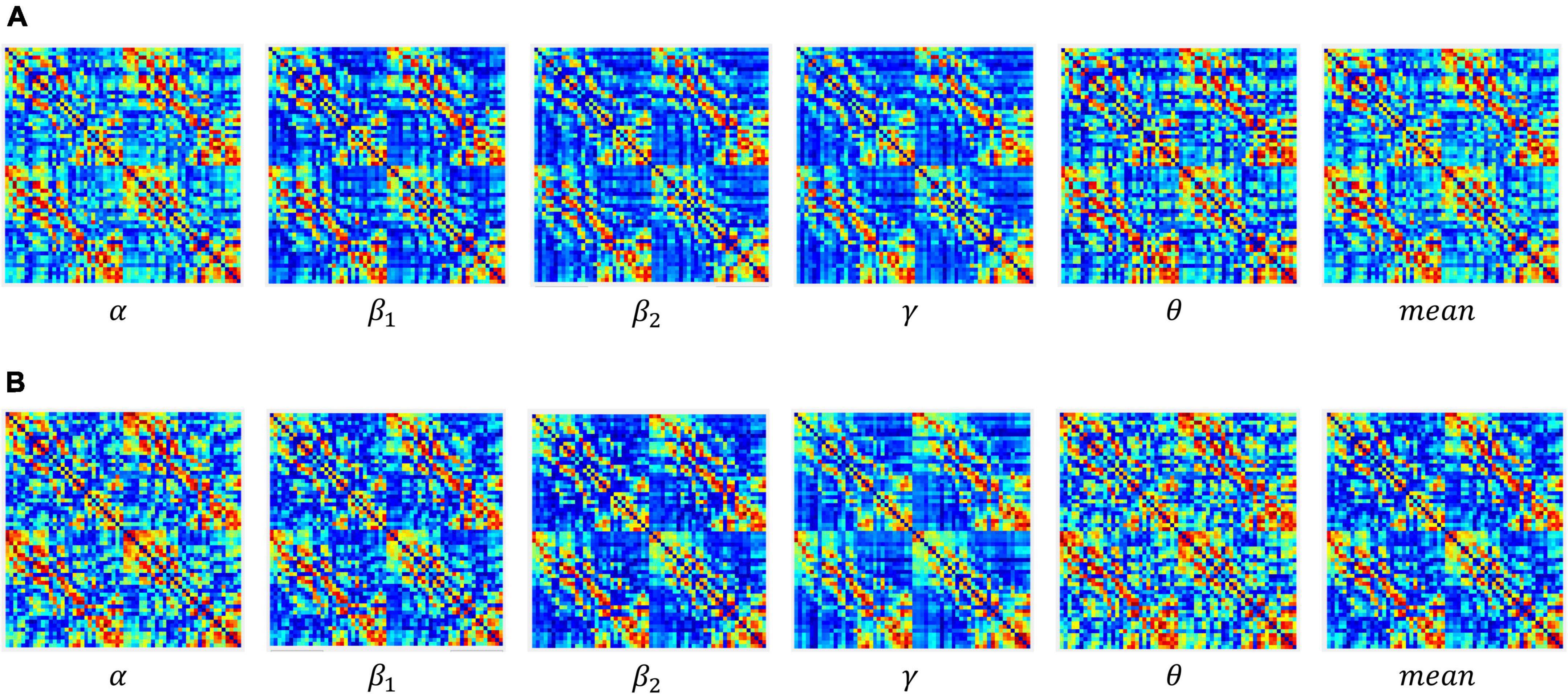
Figure 3. Adjacency matrices at different connection densities in the encoding stage: (A) control group, (B) schizophrenic patients.
Figure 3 shows that: (1) When the network connection density is small, approximately 20%, there is a significant difference in brain networks between the control group and schizophrenic patients. (2) The change in the connection matrix between the control group and schizophrenic patients gradually decreased from approximately 50% of the network connection density; this indicates that the connection matrix between the control group and schizophrenic patients in the WM coding stage had significantly different features. Moreover, the same result can be observed from the adjacency matrix constructed without the threshold in Figure 4.
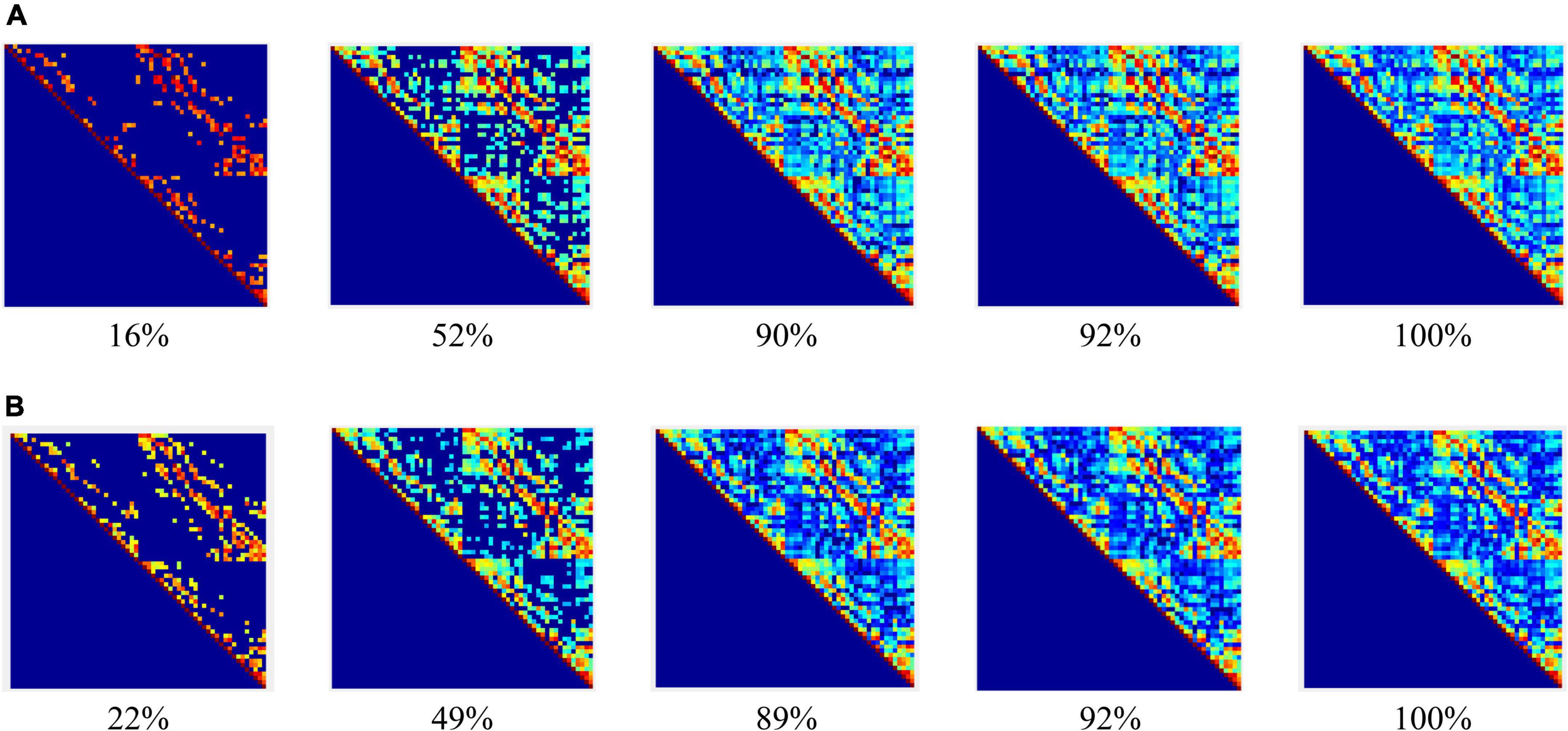
Figure 4. Adjacency matrices at different bands and means in the encoding stage: (A) control group, (B) schizophrenic patients.
Construction of the simple complex in schizophrenia task-based data
We used the JavaPlex1 software package developed by the topology computing group of Stanford University Based on PLEX library. To construct a complex, the following four parameters must be determined. (1) The point clouds coordinate file (.txt), constructed by the edge weight matrix. (2) Maximum filtering threshold ε. (3) Maximum dimension εmax. (4) Number of filtering steps (Fs). These parameters were determined according to the experimental conditions to achieve the best experimental results.
Construction of point clouds coordinate file from the edge weight matrix
First, the adjacency matrix was transformed into an edge weight matrix with each row of “ijωij.” Next, the high-dimensional matrix that represents the distance between two nodes was mapped to the low-dimensional matrix using the ISOMAP algorithm (Chen et al., 2018). Accordingly, the distance between two points was equal to their distance in the high-dimensional matrix after dimensionality reduction and a group of new sample points were found in the low-dimensional matrix. The ISOMAP algorithm preserves the geometric structure of non-linear data and maintains the global structural information.
The dimensions of 60 × 60 adjacency matrices of the control group and schizophrenic patients in full band and other five bands were reduced and reconstructed using the ISOMAP algorithm; the results are shown in Figure 5.
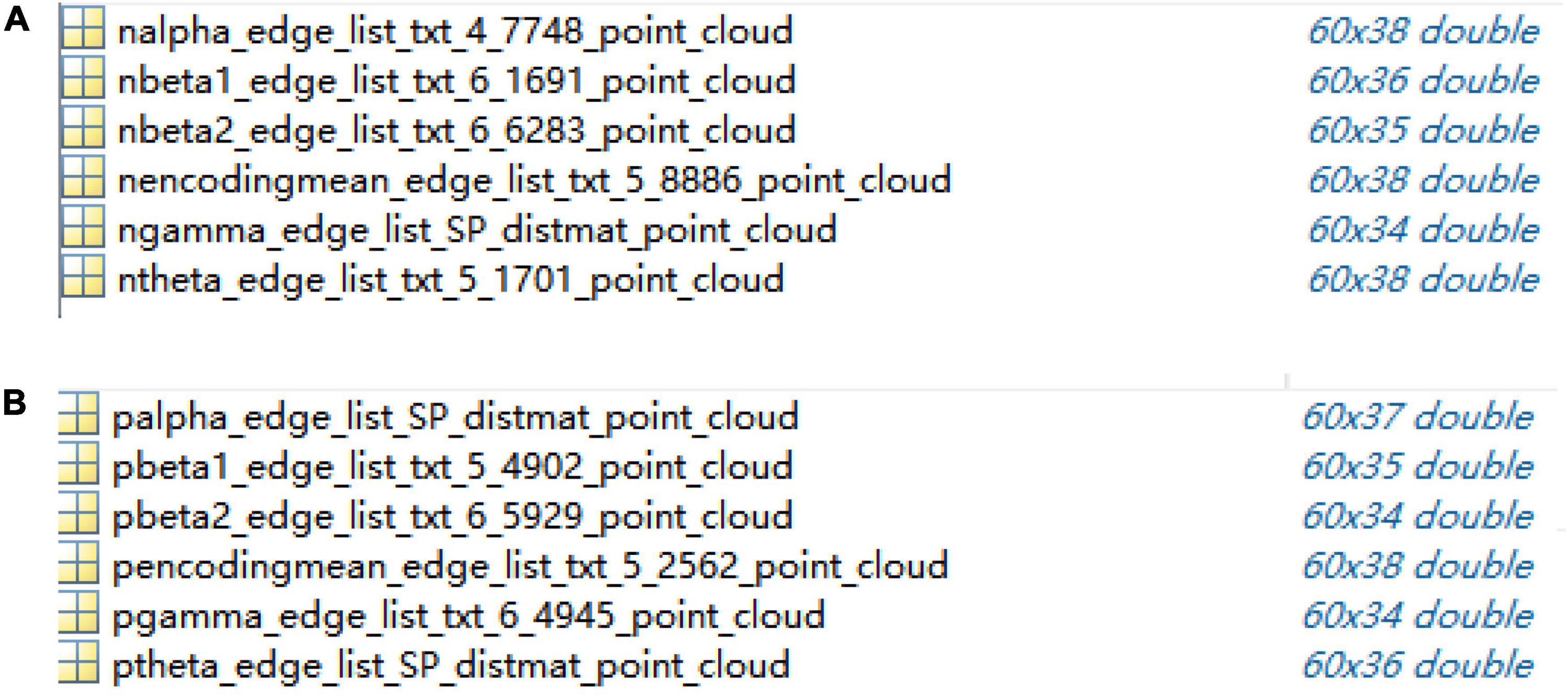
Figure 5. Point clouds from adjacency matrices through ISOMAP algorithm in encoding stage: (A) control group, (B) schizophrenic patients.
Maximum filtering threshold ε
After constructing the edge weight matrix, the maximum distance between nodes in each stage was used as the maximum filtering threshold in this experiment. The maximum filtering thresholds in the full band and five bands are listed in Table 2.
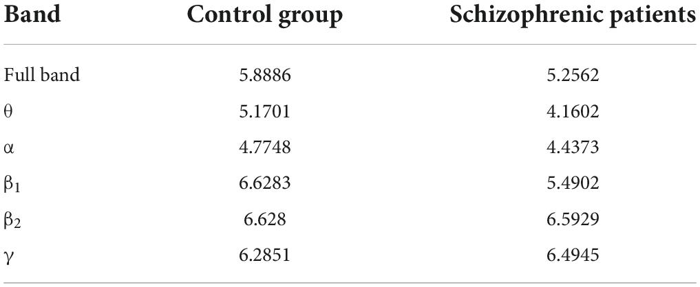
Table 2. Max filtering threshold εmax.
Dimension and number of Fs
The complex numbers: running time, dimension0 (Dim0), dimension1 (Dim1), dimension2 (Dim2), and dimension3 (Dim3) persistent feature numbers constructed in the three stages were compared. Herein, Dim0 simplex is the connected components, Dim1 simplex is the tunnels, Dim2 simplex is voids, and Dim3 simplex is three-dimensional triangle. An example of an N-dimensional simplex is shown in Figure 6.
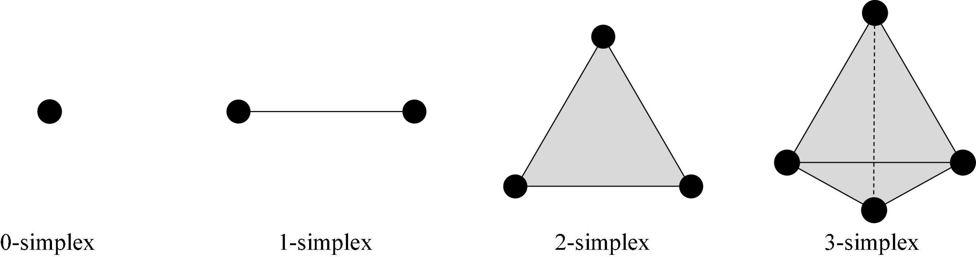
Figure 6. Example of complex.
We set the initial value of the maximum dimension to 3; that is, the persistent topological features were extracted in the four dimensions of Dim0, Dim1, Dim2, and Dim3. The number of Fs was the size of Fs. According to literature (Otter et al., 2017), Fs is usually set to 20. In this experiment, Fs was set as 20, 100, and 1000 to extract the persistent topological features and determine the optimal Fs in the model. The experimental results are summarized in Table 3.
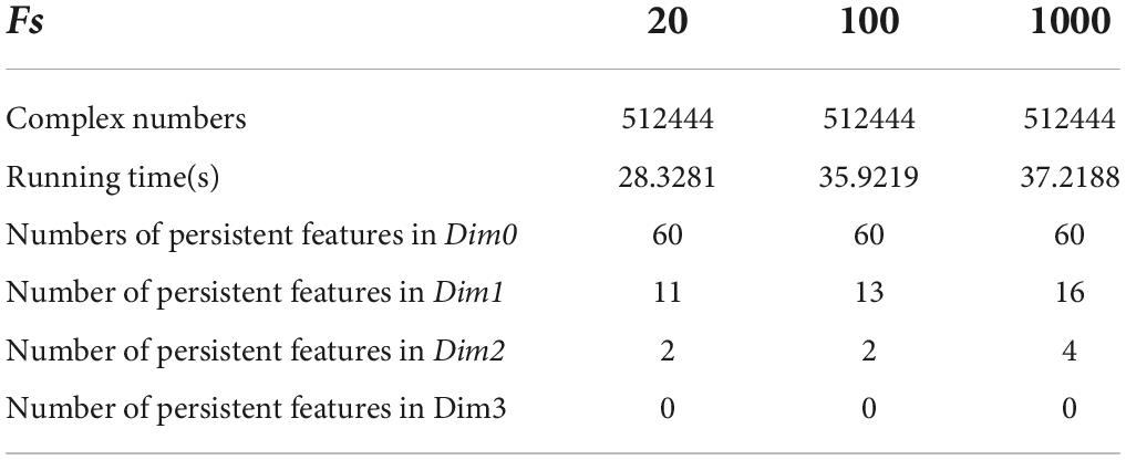
Table 3. Experimental results in three Fs.
The running time in Table 3 was obtained using a computer configured as CPU with specifications: Intel (R) core (TM) i7-6700, 32 GB memory, and Windows x64 bit operating system. The data presented in Table 3 shows that the total number of complexes constructed in the three cases remained unchanged. The running time when Fs was set as 100 was 21.14% longer than that when Fs was set as 20; however, the number of features did not change significantly. In addition, when Fs was 1000, the running time was 3.49% more than 100 and the number of features changed significantly. Therefore, to weigh the time efficiency and the number of features, Fs can be 20, 100, or 1000 when the amount of data is large. The final Fs was determined by visualizing persistence diagrams. Figures 7–9 show the persistent topological features of the control group when Fs were selected as 20, 100, and 1000.
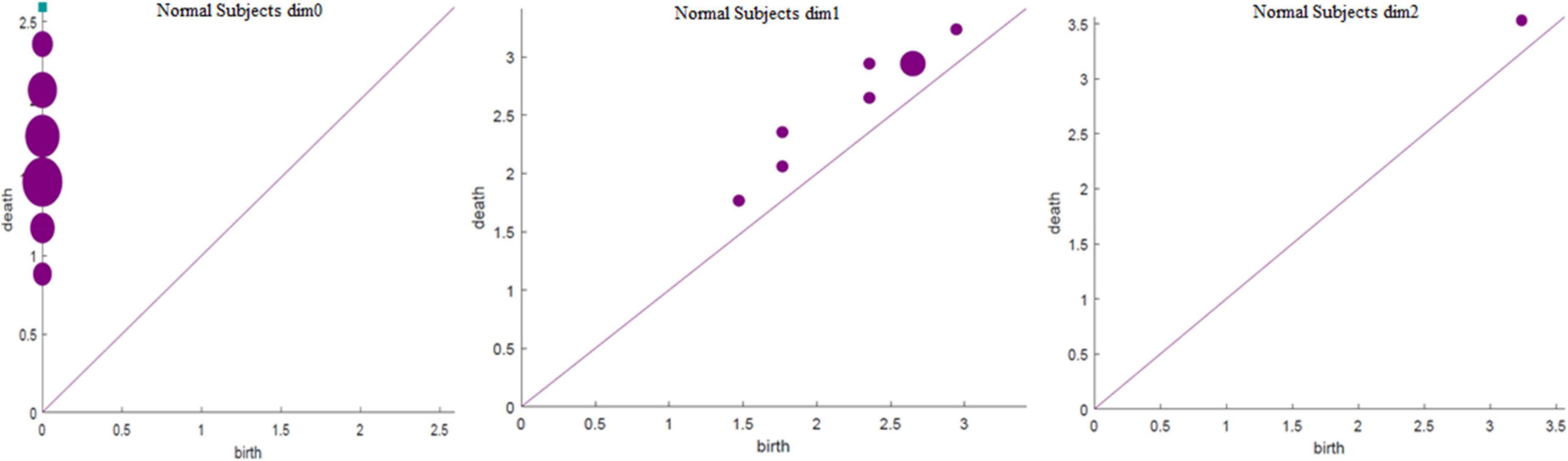
Figure 7. Persistence diagrams (Fs = 20) of the coding stage of the control group.
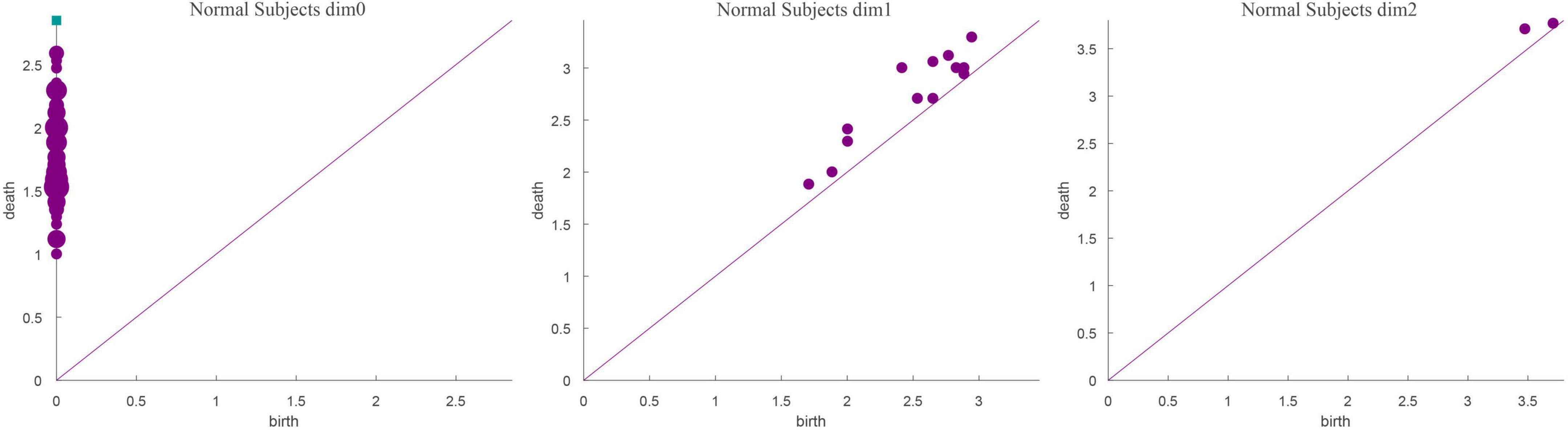
Figure 8. Persistence diagrams (Fs = 100) of the coding stage of the control group.
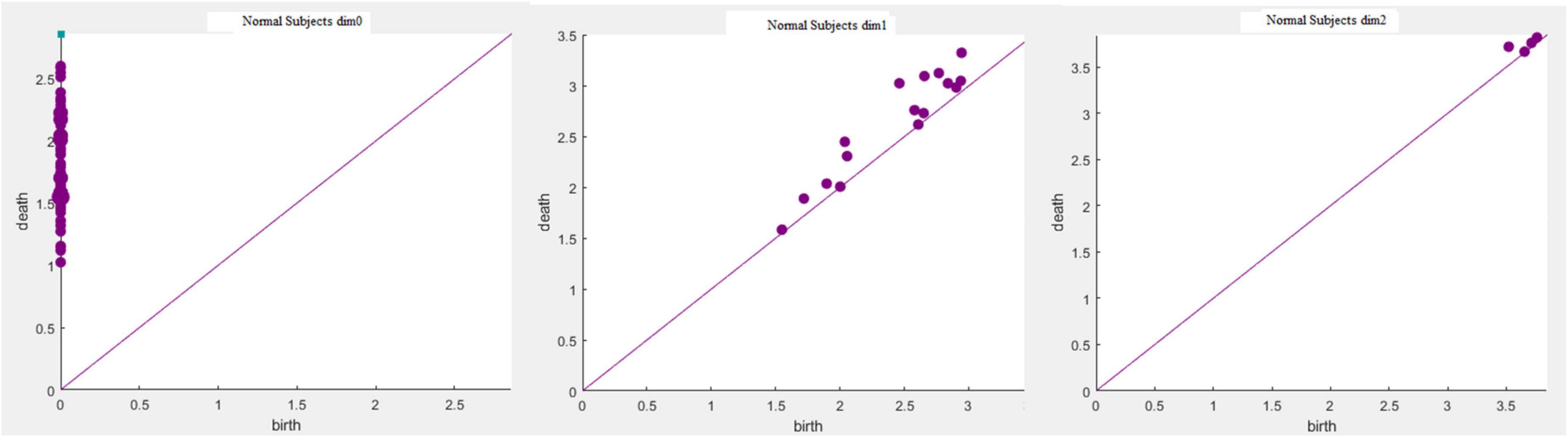
Figure 9. Persistence diagrams (Fs = 1000) of the coding stage of the control group.
Persistent topological features in schizophrenia patients
Based on the above experimental conclusions, the optimal parameters are as follows. (1) The maximum dimension was 2. (2) The maximum filtering threshold εmax of the control group and schizophrenic patients in each band were the values corresponding to those presented in Table 2. (3) The optimal Fs was 20. The persistent features of the brain network in the full band and five bands can be extracted and visualized by barcodes and persistence diagrams, respectively. The barcodes of the full band persistent features of schizophrenic patients and the control group in the coding stage are shown in Figures 10, 11.
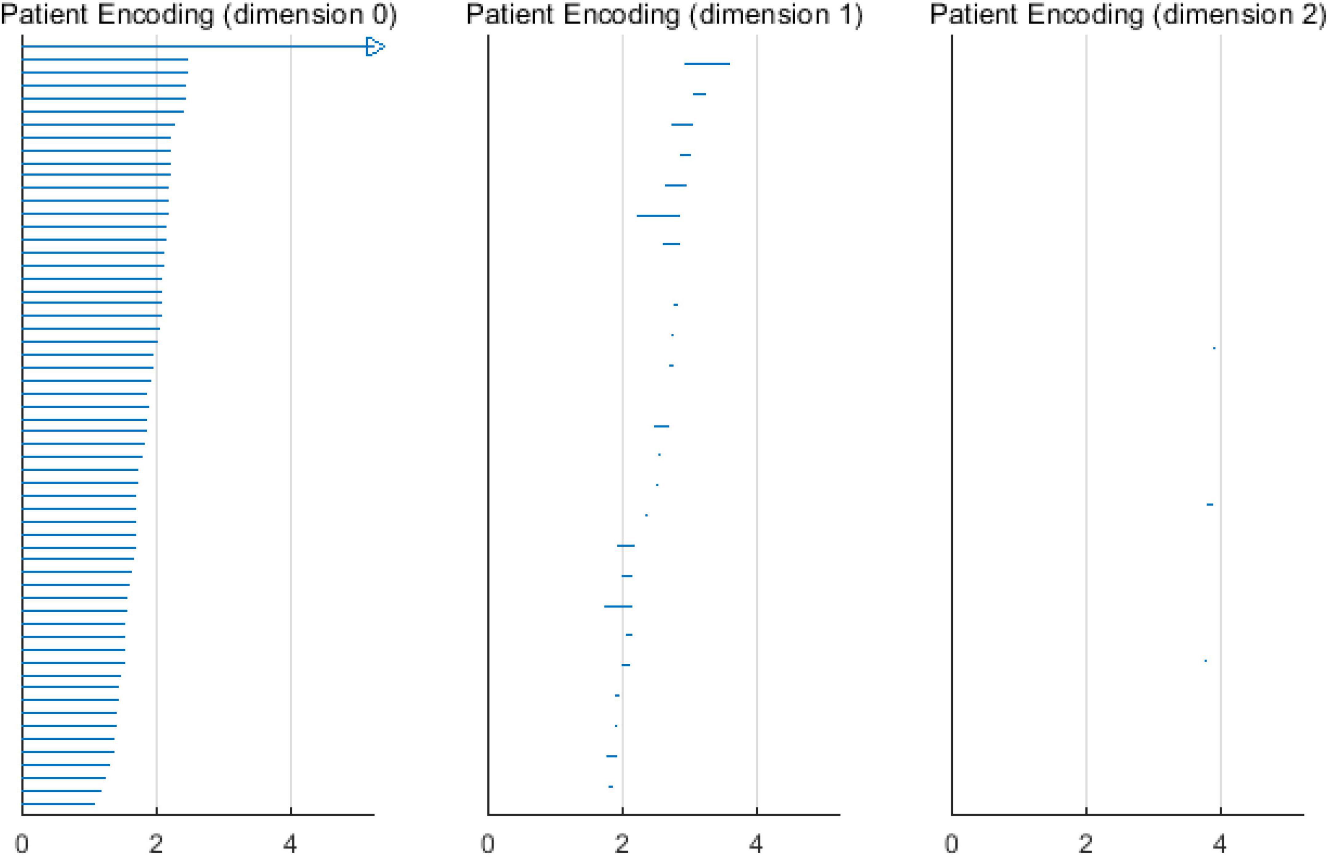
Figure 10. Barcodes of three dimensions in schizophrenic patients coding stage.
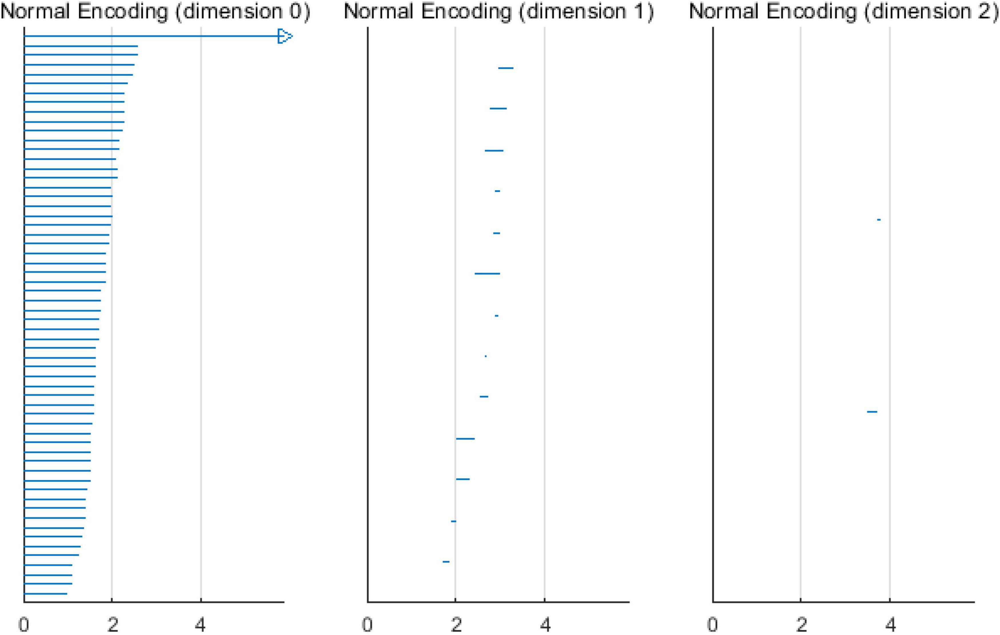
Figure 11. Barcodes of three dimensions in the control group coding stage.
Figures 7–9 show that the features of Dim0 are the same. For Dim1 and Dim2, when Fs was selected as 100 and 1000, although the number of features was greater than that when Fs was 20, most of the features that were distributed near the diagonal in Figures 8, 9 were noise. Only those that existed in the interval of [3.474274, 3.709818] were persistent topological features. Therefore, the optimal value of Fs was 20. Moreover, the data presented in Table 3 shows that the number of features of Dim3 was always zero; thus, the maximum dimension of filtering was 2.
Stability analysis of persistent topological features in schizophrenia patients
In this experiment, we used the Bottleneck distance and Wasserstein distance as metrics to compare the persistence diagrams and measure the stability of persistent features. The bottleneck distance and Wasserstein distance were calculated using the GUDHI package in Ripser in the Python environment.
Bottleneck distance
The important parameter for calculating the Bottleneck distance is accuracy e, which was set as 0.01 to calculate the approximate value; additionally, the same value of 0.01 was set as the default value to calculate the real value. A comparison of the calculation results is presented in Table 4.
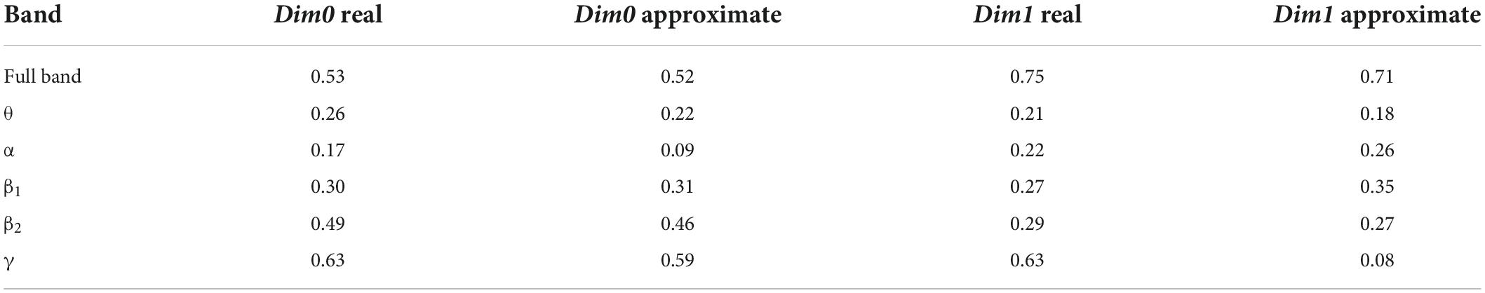
Table 4. Bottleneck distances between persistence diagrams.
The data presented in Table 4 shows that except for band α of Dim0 and band γ of Dim1, the errors between the approximate value and real value were very small; further, there may be singular values in the persistent topological features of the two bands.
Wasserstein distance
The results of the Wasserstein distance of the Dim0 and Dim1 dimensions in the full band and the five bands of the control group and schizophrenic patients are presented in Table 5.
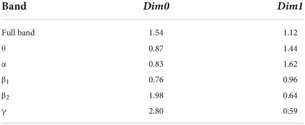
Table 5. Wasserstein distances between persistence diagrams.
Results analysis
In this study, a full-scale complex brain network model was proposed and applied to the WM data analysis of schizophrenic patients, and the related parameters and algorithms of the model were selected according to the experimental analysis. The 60-dimensional matrix was dropped to between 34 and 38 by the ISOMAP algorithm when the edge weight matrix and point clouds file were exchanged, which provided a good foundation for subsequent efficient data processing.
Several important parameters were determined through an all-round experimental effect comparison, listed as follows. (1) The maximum dimension was 2. (2) Experiments showed that there were no persistent topological features in bands β2,θ, and γ of the control group, and bands β2 and γ of schizophrenic patients in Dim2. Therefore, the stability analysis required Dim0 and Dim1. (3) The maximum Fs was 20, which preserved the important features, improved the time efficiency, and eliminated noise.
For the stability analysis, the results of the Bottleneck distance between persistence diagrams revealed that the approximate value was closer to the real value when the accuracy parameter e was the default value, but there was slight difference between the two values when there was no singular value in the persistence diagrams. In addition, the Bottleneck distance in bands α and θ was small; that is, the overall change in the persistence diagrams of the control group and schizophrenic patients was not significant. Therefore, the output of the model can be a persistent topological feature of the two bands.
Conclusion and future works
In this study, a full-scale brain network analysis model based on PH was proposed. The related algorithm and parameters in the data processing of the model were analyzed and some key problems were investigated, including the construction of nodes and edge weight matrix and the selection of filtering threshold in this network. Furthermore, the model was applied to task-based schizophrenic patients to extract persistent topological features and analyze their stability. The experimental results suggest that the full-scale brain network analysis model can be a stable biological reference standard for stability and noise immunity.
Topological data analysis can extract more hidden topological signal features, which are difficult to be decoded using general signal processing tools. Because the low-dimensional persistent features calculated by VIPs can capture noise (short survival time in barcodes and data points near the diagonal in the persistence diagrams) of the preprocessed data set; hence, the features of persistence diagrams are almost equivalent to those obtained from noiseless data. Therefore, applying PH theory to EEG brain network analysis can solve the problem of threshold selection and noise elimination.
The implicit goal of this study was to extract the topological features of the networks that persist across multiple scales in schizophrenia EEG data. However, there are some limitations to this study. First, the application of the schizophrenia EEG brain network analysis method based on PH theory in large-scale clinical EEG analysis needs further discussion and continuous research. This is required because most of the existing filtering algorithms focus on computational efficiency and cost, and rarely analyze the stability of their applications in large-scale networks. Second, although persistence diagrams are important tool in TDA, the use of machine learning algorithms in the space of persistence diagrams is challenging. One way to resolve this is by transforming the persistent diagram into a vectorized summary, which can be easily used for machine learning tasks. Some alternative representations to persistence diagrams include persistence landscapes (Bubenik, 2015; Vipond, 2020), persistence images (Adams et al., 2017; Som et al., 2020), Betti curves (Giusti et al., 2015; Curto et al., 2021), thermonuclear (Reininghaus et al., 2015), and persistence entropy (Chintakunta et al., 2015; Atienza et al., 2020). Applying these transformed features to popular machine learning methods is another work that our groups are carrying out; herein, persistent topological features are extracted using adaptive thresholding during the persistent homology filtrations. The distribution state of these features are represented by heatmaps and persistence entropies. The process states of persistent feature generation are interpreted by Betti curves and persistence landscapes. Finally, the amount of calculation of high-dimensional data filtered by the Vietoris-Rips algorithm is high and increases exponentially. Dynamic determination of the Vietoris-Rips filtering threshold ε, which significantly saves calculation time and improves the efficiency of analysis compared with the well-established approaches, will be used in our next study.
Data availability statement
The original contributions presented in the study are included in the article/supplementary material, further inquiries can be directed to the corresponding authors.
Ethics statement
The studies involving human participants were reviewed and approved by Beijing Huilongguan Hospital Ethics Committee. The patients/participants provided their written informed consent to participate in this study.
Author contributions
GG and YZ designed the study. YZ, JH, and ST acquired the data and completed data pre-processing work. CL, XX, and LJ analyzed and interpreted the results of the data analysis. GG and GY drafted the manuscript. YD, YF, DS, and LW revised the manuscript. All authors contributed to the article and approved the submitted version.
Funding
This work was supported by the National Natural Science Foundation of China (No. 61906130), the National Natural Science Foundation of Beijing (No. 7202072), Beijing Hospital Authority Enhancement Program (No. DFL20192001), the Taiyuan Normal University Graduate Education Innovation Project (No. SYYJSJC-2270), and the Postgraduate Education Innovation Project in Shanxi Province in 2022 (No. 2022Y757).
Acknowledgments
Appreciation is owed to the patients, clinical psychiatrists, and nursing staff in Beijing Huilongguang Hospital for their participation and collaboration. We also thank Edmund F. and Rhoda E. Perozzi, for helpful advice and extensive editing. We would like to thank Editage (www.editage.cn) for English language editing.
Conflict of interest
The authors declare that the research was conducted in the absence of any commercial or financial relationships that could be construed as a potential conflict of interest.
Publisher’s note
All claims expressed in this article are solely those of the authors and do not necessarily represent those of their affiliated organizations, or those of the publisher, the editors and the reviewers. Any product that may be evaluated in this article, or claim that may be made by its manufacturer, is not guaranteed or endorsed by the publisher.
Footnotes
- ^ JavaPlex[EB/OL]. http://appliedtopology.github.io/javaplex/.
References
Adams, H., Emerson, T., Kirby, M., Neville, R., Peterson, C., Shipman, P., et al. (2017). Persistence images: A stable vector representation of persistent homology. J. Mach. Learn. Res. 18, 1–35.
Adler, R. J., Bobrowski, O., Borman, M. S., Subag, E., and Weinberger, S. (2010). Persistent homology for random fields and complexes. Borrowing strength: Theory powering applications–a Festschrift for Lawrence D. Brown. Inst. Math. Stat. 6, 124–143.
Agarwal, P. K., and Sharathkumar, R. (2014). “Approximation algorithms for bipartite matching with metric and geometric costs,” in Proceedings of the Forty-Sixth Annual ACM Symposium on Theory of Computing, (New York, NY: ACM Digital Library), 555–564.
Aktas, M. E., Akbas, E., and El Fatmaoui, A. (2019). Persistence homology of networks: Methods and applications. Appl. Netw. Sci. 4:61. doi: 10.1007/s41109-019-0179-3
Atienza, N., Gonzalez-Díaz, R., and Soriano-Trigueros, M. (2020). On the stability of persistent entropy and new summary functions for topological data analysis. Pattern Recognize. 107:107509. doi: 10.1016/j.patcog.2020.107509
Benesty, J., Chen, J., Huang, Y., and Cohen, I. (2009). Pearson Correlation Coefficient Noise Reduction in Speech Processing Springer Topics in Signal Processing. Berlin: Springer. doi: 10.1007/978-3-642-00296-0-5
Bubenik, P., and Dłotko, P. J. (2017). A persistence landscapes toolbox for topological statistics. J. Symb. Comput. 78, 91–114. doi: 10.1016/j.jsc.2016.03.009
Bubenik, P. (2015). Statistical topological data analysis using persistence landscapes. J. Mach. Learn. Res. 16, 77–102.
Caputi, L., Pidnebesna, A., and Hlinka, J. (2021). Promises and pitfalls of Topological Data Analysis for brain connectivity analysis. NeuroImage 238:118245. doi: 10.1016/j.neuroimage.2021.118245
Carlsson, G., Zomorodian, A., Collins, A., and Guibas, L. J. (2005). Persistence barcodes for shapes. Int. J. Shape Model. 11, 149–187. doi: 10.1142/S0218654305000761
Carlsson, G. J. (2009). Topology and data. Bull. Am. Math. Soc. 46, 255–308. doi: 10.1090/S0273-0979-09-01249-X
Castro, E., Martínez-Ramón, M., Pearlson, G., Sui, J., and Calhoun, V. D. J. N. (2011). Characterization of groups using composite kernels and multi-source fMRI analysis data: Application to schizophrenia. NeuroImage 58, 526–536. doi: 10.1016/j.neuroimage.2011.06.044
Chen, H., Perozzi, B., Al-Rfou, R., and Skiena, S. J. (2018). A tutorial on network embeddings. arXiv [Preprint]. doi: 10.48550/arXiv.1808.02590
Chintakunta, H., Gentimis, T., Gonzalez-Diaz, R., Jimenez, M.-J., and Krim, H. (2015). An entropy-based persistence barcode. Pattern Recognize. 48, 391–401. doi: 10.1016/j.patcog.2014.06.023
Choudhary, A. (2017). Approximation Algorithms for Vietoris-Rips and Čech filtrations. Germany: Saarland University.
Chung, M. K., Hanson, J. L., Ye, J., Davidson, R. J., and Pollak, S. D. (2015). Persistent homology in sparse regression and its application to brain morphometry. IEEE Trans. Med. Imaging 34, 1928–1939. doi: 10.1109/TMI.2015.2416271
Curto, C., Paik, J., and Rivin, I. (2021). “Betti Curves of Rank One Symmetric Matrices,” in Geometric Science of Information GSI 2021 Lecture Notes in Computer Science, eds F. Nielsen and F. Barbaresco (Cham: Springer), doi: 10.1007/978-3-030-80209-7-69
Edelsbrunner, H., and Harer, J. L. (2010). Computational Topology: An Introduction. Washington, DC: American Mathematical Society
Efrat, A., Itai, A., and Katz, M. (2001). Geometry helps in bottleneck matching and related problems. Algorithmica 31, 1–28. doi: 10.1007/s00453-001-0016-8
Espinoza, J. F., Hernández-Amador, R., Hernández-Hernández, H. A., and Ramonetti-Valencia, B. (2020). A numerical approach for the filtered generalized Čech complex. Algorithms 13:11. doi: 10.3390/a13010011
Ghrist, R. J. (2008). Barcodes: The persistent topology of data. Bull. Am. Math. Soc. 45, 61–75. doi: 10.1090/S0273-0979-07-01191-3
Giusti, C., Pastalkova, E., Curto, C., and Itskov, V. (2015). Clique topology reveals intrinsic geometric structure in neural correlations. Proc. Natl. Acad. Sci. U S A. 112, 13455–13460. doi: 10.1073/pnas.1506407112
Guibas, L. J., and Oudot, S. Y. (2008). Reconstruction using witness complexes. Discrete Comput. Geom. 40, 325–356. doi: 10.1007/s00454-008-9094-6
Horak, D., Maletić, S., and Rajković, M. J. (2009). Persistent homology of complex networks. arXiv [Preprint]. doi: 10.1088/1742-5468/2009/03/P03034
Huang, S.-G., Chung, M. K., Carroll, I. C., and Goldsmith, H. H. (2019). Dynamic Connectivity without Sliding Windows. arxiv [Preprint]. doi: 10.1109/dsw.2019.8755550
Ibekwe, A. M., Ma, J., Crowley, D. E., Yang, C.-H., Johnson, A. M., Petrossian, T. C., et al. (2014). Topological data analysis of Escherichia coli O157: H7 and non-O157 survival in soils. Front. Cell. Infect. Microbiol. 4:122. doi: 10.3389/fcimb.2014.00122
Jamil, F., and Kim, D. H. (2019). Improving accuracy of the alpha–beta filter algorithm using an ANN-based learning mechanism in indoor navigation system. Sensors 19:3946. doi: 10.3390/s19183946
Jin, D., Li, R., and Xu, J. (2019). Multiscale community detection in functional brain networks constructed using dynamic time warping. IEEE Trans. Neural Syst. Rehabilitation Eng. 28, 52–61. doi: 10.1109/TNSRE.2019.2948055
Jungeblut, H. M., Hagemann, D., Löffler, C., and Schubert, A.-L. (2021). An Investigation of the Slope Parameters of Reaction Times and P3 Latencies in the Sternberg Memory Scanning Task–A Fixed-Links Model Approach. J. Cogn. 4:26 doi: 10.5334/joc.158
Kay, S. R., Fiszbein, A., and Opler, L. A. (1987). The positive and negative syndrome scale (PANSS) for schizophrenia. Schizophr. Bull. 13, 261–276. doi: 10.1093/schbul/13.2.261
Kerber, M., Morozov, D., and Nigmetov, A. (2017). Geometry Helps to Compare Persistence Diagrams. New York, NY: ACM.
Khalid, A., Kim, B. S., Chung, M. K., Ye, J. C., and Jeon, D. J. N. (2014). Tracing the evolution of multi-scale functional networks in a mouse model of depression using persistent brain network homology. NeuroImage 101, 351–363. doi: 10.1016/j.neuroimage.2014.07.040
Lee, H., Kang, H., Chung, M. K., Kim, B.-N., and Lee, D. S. (2012). Persistent brain network homology from the perspective of dendrogram. IEEE Trans. Med. Imaging 31, 2267–2277. doi: 10.1109/TMI.2012.2219590
Lee, H., Ma, Z., Wang, Y., and Chung, M. K. (2017). Topological distances between networks and its application to brain imaging. arXiv [Preprint]. doi: 10.48550/arXiv.1701.04171
Li, H., and Fan, Y. (2013). Functional brain atlas construction for brain network analysis. Med. Imaging 8669:86690C
Li, W., Wang, Z., Zhang, L., Qiao, L., and Shen, D. (2017). Remodeling Pearson’s correlation for functional brain network estimation and autism spectrum disorder identification. Front. Neuroinform. 11:55. doi: 10.3389/fninf.2017.00055
Li, Z., Zhang, L., Zhang, F., Gu, R., Peng, W., and Hu, L. (2020). Demystifying signal processing techniques to extract resting-state EEG features for psychologists. Brain Neurosci. Adv. 6, 189–209. doi: 10.26599/BSA.2020.9050019
Manoach, D. S., Press, D. Z., Thangaraj, V., Searl, M. M., Goff, D. C., Halpern, E., et al. (1999). Schizophrenic subjects activate dorsolateral prefrontal cortex during a working memory task, as measured by fMRI. Biol. Psychiatry 45, 1128–1137. doi: 10.1016/S0006-3223(98)00318-7
Otter, N., Porter, M. A., Tillmann, U., Grindrod, P., and Harrington, H. A. (2017). A roadmap for the computation of persistent homology. EPJ Data Sci. 6:17. doi: 10.1140/epjds/s13688-017-0109-5
Reininghaus, J., Huber, S., Bauer, U., and Kwitt, R. (2015). “A stable multi-scale kernel for topological machine learning,” in Proceedings of the IEEE Conference on Computer Vision and Pattern Recognition, (New York, NY: IEEE), 4741–4748. doi: 10.3389/frai.2021.681174
Segal, D. L. (2010). “Diagnostic and statistical manual of mental disorders (DSM-IV-TR),” in The Corsini Encyclopedia of Psychology (p. corpsy0271), eds I. B. Weiner and W. E. Craighead (Hoboken: John Wiley Sons, Inc.), 1–3. doi: 10.1002/9780470479216.corpsy0271
Shnier, D., Voineagu, M. A., and Voineagu, I. (2019). Persistent homology analysis of brain transcriptome data in autism. J. R. Soc. Interface 16:20190531. doi: 10.1098/rsif.2019.0531
Sizemore, A. E., Giusti, C., Kahn, A., Vettel, J. M., Betzel, R. F., and Bassett, D. S. (2018). Cliques and cavities in the human connectome. J. Comput. Neurosci. 44, 115–145. doi: 10.1007/s10827-017-0672-6
Som, A., Choi, H., Ramamurthy, K. N., Buman, M. P., and Turaga, P. (2020). Pi-net: A deep learning approach to extract topological persistence images. Conf. Comput. Vis. Pattern Recognit. Workshops 2020, 834–835. doi: 10.1109/cvprw50498.2020.00425
Taylor, D., Klimm, F., Harrington, H. A., Kramár, M., Mischaikow, K., Porter, M. A., et al. (2015). Topological data analysis of contagion maps for examining spreading processes on networks. Nat. Commun. 6:7723. doi: 10.1038/ncomms8723
Telesford, Q. K., Simpson, S. L., Burdette, J. H., Hayasaka, S., and Laurienti, P. J. (2011). The brain as a complex system: Using network science as a tool for understanding the brain. Brain Connect. 1, 295–308. doi: 10.1089/brain.2011.0055
Tewarie, P., van Dellen, E., Hillebrand, A., and Stam, C. J. (2015). The minimum spanning tree: An unbiased method for brain network analysis. NeuroImage 104, 177–188. doi: 10.1016/j.neuroimage.2014.10.015
van Wijk, B. C., Stam, C. J., and Daffertshofer, A. (2010). Comparing brain networks of different size and connectivity density using graph theory. PLoS One 5:e13701. doi: 10.1371/journal.pone.0013701
Vipond, O. (2020). Multiparameter Persistence Landscapes. J. Mach. Learn. Res. 21, 1–38. doi: 10.1073/pnas.2102166118
Xu, X., Drougard, N., and Roy, R. N. (2021). Topological Data Analysis as a New Tool for EEG Processing. Front. Neurosci. 15:761703. doi: 10.3389/fnins.2021.761703
Yin, G., Li, H., Tan, S., Yao, R., Cui, X., and Zhao, L. J. (2020). Synchronization Stability Model of Complex Brain Networks: An EEG Study. Front. Psychiatry 11:1226. doi: 10.3389/fpsyt.2020.571068
Young, J.-G., Petri, G., Vaccarino, F., and Patania, A. J. (2017). Construction of and efficient sampling from the simplicial configuration model. Phys. Rev. E 96:032312. doi: 10.1103/PhysRevE.96.032312
Zalesky, A., Fornito, A., Egan, G. F., Pantelis, C., and Bullmore, E. T. (2012). The relationship between regional and inter-regional functional connectivity deficits in schizophrenia. Hum. Brain Mapp. 33, 2535–2549. doi: 10.1002/hbm.21379
Zavlanos, M. M., Spesivtsev, L., and Pappas, G. J. (2008). “A distributed auction algorithm for the assignment problem,” in 2008 47th IEEE Conference on Decision and Control), (New York, NY: IEEE), 1212–1217. doi: 10.1109/CDC.2008.4739098
Zhu, J., Qian, Y., Zhang, B., Li, X., Bai, Y., Li, X., et al. (2020). Abnormal synchronization of functional and structural networks in schizophrenia. Brain Imaging Behav. 14, 2232–2241. doi: 10.1007/s11682-019-00175-8
Zomorodian, A., and Carlsson, G. (2005). Computing persistent homology. Discrete Comput. Geom. 33, 249–274. doi: 10.1007/s00454-004-1146-y
Keywords: topological data analysis, persistent homology, complex brain networks, schizophrenia patients, persistent topological features, EEG signal
Citation: Guo G, Zhao Y, Liu C, Fu Y, Xi X, Jin L, Shi D, Wang L, Duan Y, Huang J, Tan S and Yin G (2022) Method for persistent topological features extraction of schizophrenia patients’ electroencephalography signal based on persistent homology. Front. Comput. Neurosci. 16:1024205. doi: 10.3389/fncom.2022.1024205
Received: 21 August 2022; Accepted: 21 September 2022;
Published: 05 October 2022.
Edited by:
Bin Wang, Taiyuan University of Technology, ChinaReviewed by:
Chunlin Li, Capital Medical University, ChinaXiaoyu Tang, Liaoning Normal University, China
Copyright © 2022 Guo, Zhao, Liu, Fu, Xi, Jin, Shi, Wang, Duan, Huang, Tan and Yin. This is an open-access article distributed under the terms of the Creative Commons Attribution License (CC BY). The use, distribution or reproduction in other forums is permitted, provided the original author(s) and the copyright owner(s) are credited and that the original publication in this journal is cited, in accordance with accepted academic practice. No use, distribution or reproduction is permitted which does not comply with these terms.
*Correspondence: Shuping Tan, shupingtan@126.com; Guimei Yin, yinguimeicn@126.com
†These authors have contributed equally to this work